Im Assuming Arch Is First but Then Again

How to Model Volatility with ARCH and GARCH for Time Serial Forecasting in Python

Last Updated on August 21, 2019

A alter in the variance or volatility over time can cause problems when modeling time series with classical methods similar ARIMA.

The Arch or Autoregressive Conditional Heteroskedasticity method provides a way to model a change in variance in a time series that is time dependent, such as increasing or decreasing volatility. An extension of this approach named GARCH or Generalized Autoregressive Conditional Heteroskedasticity allows the method to support changes in the time dependent volatility, such as increasing and decreasing volatility in the same series.

In this tutorial, you volition discover the Curvation and GARCH models for predicting the variance of a fourth dimension series.

Later on completing this tutorial, you will know:

The problem with variance in a time series and the need for ARCH and GARCH models.
How to configure ARCH and GARCH models.
How to implement Curvation and GARCH models in Python.

Kicking-start your project with my new book Time Serial Forecasting With Python, including step-past-step tutorials and the Python source code files for all examples.

Permit's get started.

How to Develop Arch and GARCH Models for Fourth dimension Series Forecasting in Python
Photo by Murray Foubister, some rights reserved.

Tutorial Overview

This tutorial is divided into five parts; they are:

Problem with Variance
What Is an ARCH Model?
What Is a GARCH Model?
How to Configure ARCH and GARCH Models
Curvation and GARCH Models in Python

Trouble with Variance

Autoregressive models can exist adult for univariate time series data that is stationary (AR), has a tendency (ARIMA), and has a seasonal component (SARIMA).

One aspect of a univariate time series that these autoregressive models do not model is a change in the variance over time.

Classically, a fourth dimension series with small-scale changes in variance can sometimes be adjusted using a ability transform, such equally by taking the Log or using a Box-Cox transform.

In that location are some time series where the variance changes consistently over time. In the context of a fourth dimension series in the financial domain, this would be called increasing and decreasing volatility.

In time series where the variance is increasing in a systematic way, such every bit an increasing trend, this property of the series is called heteroskedasticity. Information technology'southward a fancy discussion from statistics that means changing or unequal variance across the series.

If the modify in variance tin be correlated over time, then it tin exist modeled using an autoregressive process, such as Arch.

What Is an ARCH Model?

Autoregressive Conditional Heteroskedasticity, or Arch, is a method that explicitly models the modify in variance over fourth dimension in a time serial.

Specifically, an Arch method models the variance at a time step equally a function of the rest errors from a mean process (e.yard. a cypher mean).

The Curvation process introduced by Engle (1982) explicitly recognizes the divergence between the unconditional and the conditional variance assuasive the latter to modify over time equally a part of by errors.

— Generalized autoregressive conditional heteroskedasticity, 1986.

A lag parameter must exist specified to define the number of prior residual errors to include in the model. Using the note of the GARCH model (discussed later), we can refer to this parameter as "q". Originally, this parameter was called "p", and is also called "p" in the arch Python package used later in this tutorial.

q: The number of lag squared residue errors to include in the Curvation model.

A generally accepted notation for an Curvation model is to specify the Arch() function with the q parameter ARCH(q); for case, ARCH(i) would be a first guild Curvation model.

The approach expects the series is stationary, other than the change in variance, meaning information technology does not accept a trend or seasonal component. An ARCH model is used to predict the variance at future time steps.

[Arch] are mean zero, serially uncorrelated processes with nonconstant variances conditional on the past, simply constant unconditional variances. For such processes, the recent past gives data near the one-menstruum forecast variance.

– Autoregressive Provisional Heteroscedasticity with Estimates of the Variance of U.k. Inflation, 1982.

In practice, this can be used to model the expected variance on the residuals later on some other autoregressive model has been used, such as an ARMA or similar.

The model should only be practical to a prewhitened balance series {e_t} that is uncorrelated and contains no trends or seasonal changes, such as might be obtained later fitting a satisfactory SARIMA model.

— Page 148, Introductory Time Series with R, 2009.

What Is a GARCH Model?

Generalized Autoregressive Conditional Heteroskedasticity, or GARCH, is an extension of the ARCH model that incorporates a moving average component together with the autoregressive component.

Specifically, the model includes lag variance terms (east.g. the observations if modeling the white noise residuum errors of another process), together with lag residual errors from a mean process.

The introduction of a moving average component allows the model to both model the conditional change in variance over time likewise as changes in the time-dependent variance. Examples include conditional increases and decreases in variance.

Equally such, the model introduces a new parameter "p" that describes the number of lag variance terms:

p: The number of lag variances to include in the GARCH model.
q: The number of lag residual errors to include in the GARCH model.

A by and large accepted notation for a GARCH model is to specify the GARCH() part with the p and q parameters GARCH(p, q); for example GARCH(1, 1) would exist a first order GARCH model.

A GARCH model subsumes Curvation models, where a GARCH(0, q) is equivalent to an Arch(q) model.

For p = 0 the process reduces to the ARCH(q) procedure, and for p = q = 0 E(t) is simply white racket. In the ARCH(q) process the conditional variance is specified as a linear part of past sample variances only, whereas the GARCH(p, q) process allows lagged conditional variances to enter every bit well. This corresponds to some sort of adaptive learning mechanism.

— Generalized autoregressive conditional heteroskedasticity, 1986.

As with Arch, GARCH predicts the future variance and expects that the series is stationary, other than the change in variance, meaning information technology does non have a trend or seasonal component.

How to Configure Arch and GARCH Models

The configuration for an Arch model is best understood in the context of ACF and PACF plots of the variance of the time series.

This tin exist achieved by subtracting the hateful from each ascertainment in the serial and squaring the consequence, or just squaring the observation if you're already working with white noise residuals from some other model.

If a correlogram appears to exist white noise […], then volatility ca be detected by looking at the correlogram of the squared values since the squared values are equivalent to the variance (provided the series is adjusted to have a mean of zilch).

— Pages 146-147, Introductory Time Series with R, 2009.

The ACF and PACF plots can so be interpreted to guess values for p and q, in a similar way as is washed for the ARMA model.

For more information on how to practice this, see the post:

A Gentle Introduction to Autocorrelation and Partial Autocorrelation

ARCH and GARCH Models in Python

In this section, nosotros volition look at how nosotros can develop ARCH and GARCH models in Python using the arch library.

First, let's set up a dataset nosotros can utilise for these examples.

Exam Dataset

We can create a dataset with a controlled model of variance.

The simplest case would exist a series of random dissonance where the mean is goose egg and the variance starts at 0.0 and steadily increases.

Nosotros can accomplish this in Python using the gauss() function that generates a Gaussian random number with the specified mean and standard deviation.

# create dataset

data = [ gauss ( 0 , i* 0.01 ) for i in range ( i , 100 + 1 ) ]

Nosotros can plot the dataset to get an idea of how the linear change in variance looks. The complete example is listed below.

# create a simple white noise with increasing variance

from random import gauss

from random import seed

from matplotlib import pyplot

# seed pseudorandom number generator

seed ( 1 )

# create dataset

data = [ gauss ( 0 , i* 0.01 ) for i in range ( 0 , 100 ) ]

# plot

pyplot . plot ( data )

pyplot . prove ( )

Running the example creates and plots the dataset. Nosotros can see the clear change in variance over the course of the series.

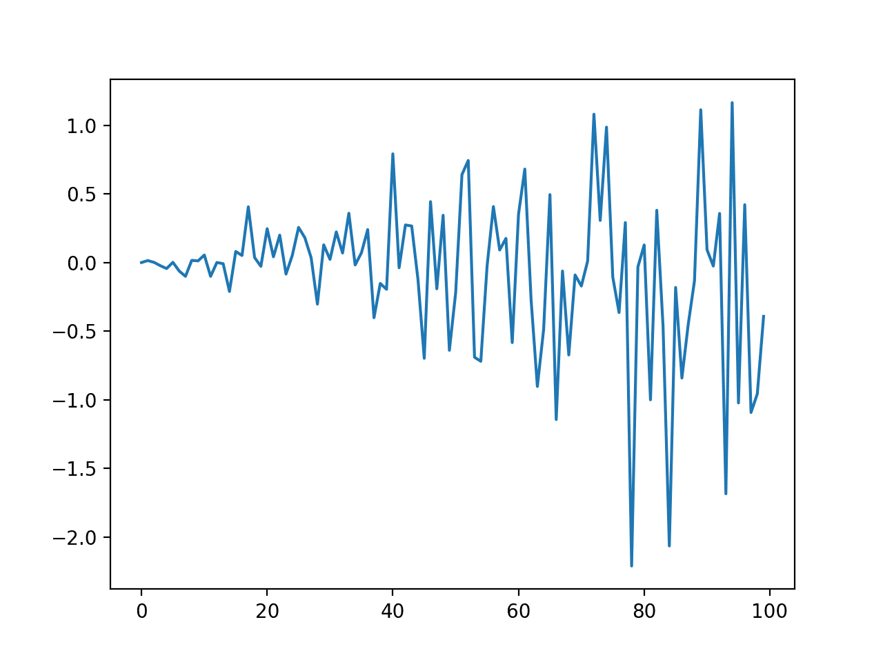
Line Plot of Dataset with Increasing Variance

Autocorrelation

We know there is an autocorrelation in the variance of the contrived dataset.

Nevertheless, we can look at an autocorrelation plot to confirm this expectation. The complete example is listed below.

# bank check correlations of squared observations

from random import gauss

from random import seed

from matplotlib import pyplot

from statsmodels . graphics . tsaplots import plot _acf

# seed pseudorandom number generator

seed ( 1 )

# create dataset

data = [ gauss ( 0 , i* 0.01 ) for i in range ( 0 , 100 ) ]

# foursquare the dataset

squared_data = [ x* * 2 for x in data ]

# create acf plot

plot_acf ( squared_data )

pyplot . prove ( )

Running the example creates an autocorrelation plot of the squared observations. We run across significant positive correlation in variance out to maybe 15 lag time steps.

This might brand a reasonable value for the parameter in the ARCH model.

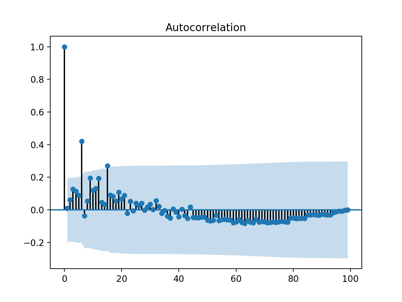
Autocorrelation Plot of Information with Increasing Variance

ARCH Model

Developing an Curvation model involves three steps:

Define the model
Fit the model
Make a forecast.

Earlier fitting and forecasting, we can split the dataset into a train and test set and then that we can fit the model on the train and evaluate its performance on the exam set up.

# split into train/exam

n_test = 10

train , test = data [ : - n_test ] , data [ - n_test : ]

A model can exist defined by calling the arch_model() function. We can specify a model for the mean of the series: in this example mean='Zip' is an appropriate model. We can and so specify the model for the variance: in this example vol='Curvation'. We tin can likewise specify the lag parameter for the ARCH model: in this instance p=15.

Note, in the arch library, the names of p and q parameters for ARCH/GARCH have been reversed.

# define model

model = arch_model ( railroad train , mean = 'Zero' , vol = 'Curvation' , p = 15 )

The model can be fit on the data past calling the fit() function. In that location are many options on this part, although the defaults are good enough for getting started. This will return a fit model.

# fit model

model_fit = model . fit ( )

Finally, we can make a prediction by calling the forecast() function on the fit model. We can specify the horizon for the forecast.

In this example, we will predict the variance for the last x time steps of the dataset, and withhold them from the grooming of the model.

# forecast the test set

yhat = model_fit . forecast ( horizon = n_test )

We tin can tie all of this together; the complete example is listed below.

two

xiv

xvi

twenty

# example of ARCH model

from random import gauss

from random import seed

from matplotlib import pyplot

from curvation import curvation _model

# seed pseudorandom number generator

seed ( 1 )

# create dataset

information = [ gauss ( 0 , i* 0.01 ) for i in range ( 0 , 100 ) ]

# split up into railroad train/test

n_test = 10

train , examination = data [ : - n_test ] , information [ - n_test : ]

# ascertain model

model = arch_model ( train , mean = 'Zero' , vol = 'ARCH' , p = 15 )

# fit model

model_fit = model . fit ( )

# forecast the test set

yhat = model_fit . forecast ( horizon = n_test )

# plot the bodily variance

var = [ i* 0.01 for i in range ( 0 , 100 ) ]

pyplot . plot ( var [ - n_test : ] )

# plot forecast variance

pyplot . plot ( yhat . variance . values [ - i , : ] )

pyplot . show ( )

Running the instance defines and fits the model then predicts the variance for the last x time steps of the dataset.

A line plot is created comparing the series of expected variance to the predicted variance. Although the model was not tuned, the predicted variance looks reasonable.

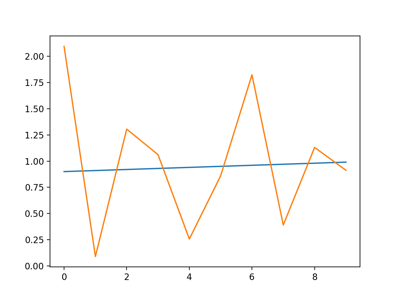
Line Plot of Expected Variance to Predicted Variance using Curvation

GARCH Model

We tin can fit a GARCH model simply as easily using the curvation library.

The arch_model() office tin can specify a GARCH instead of Curvation model vol='GARCH' likewise as the lag parameters for both.

# ascertain model

model = arch_model ( railroad train , hateful = 'Zero' , vol = 'GARCH' , p = 15 , q = 15 )

The dataset may not be a good fit for a GARCH model given the linearly increasing variance, even so, the complete instance is listed below.

vii

xiii

xiv

xviii

# case of ARCH model

from random import gauss

from random import seed

from matplotlib import pyplot

from curvation import arch _model

# seed pseudorandom number generator

seed ( 1 )

# create dataset

data = [ gauss ( 0 , i* 0.01 ) for i in range ( 0 , 100 ) ]

# divide into train/examination

n_test = x

train , test = data [ : - n_test ] , data [ - n_test : ]

# define model

model = arch_model ( train , mean = 'Zilch' , vol = 'GARCH' , p = 15 , q = 15 )

# fit model

model_fit = model . fit ( )

# forecast the examination prepare

yhat = model_fit . forecast ( horizon = n_test )

# plot the bodily variance

var = [ i* 0.01 for i in range ( 0 , 100 ) ]

pyplot . plot ( var [ - n_test : ] )

# plot forecast variance

pyplot . plot ( yhat . variance . values [ - ane , : ] )

pyplot . testify ( )

A plot of the expected and predicted variance is listed beneath.

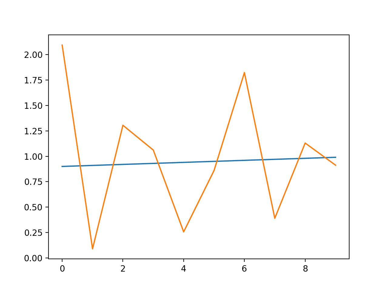
Line Plot of Expected Variance to Predicted Variance using GARCH

Summary

In this tutorial, you lot discovered the ARCH and GARCH models for predicting the variance of a time series.

Specifically, yous learned:

The trouble with variance in a fourth dimension serial and the need for ARCH and GARCH models.
How to configure ARCH and GARCH models.
How to implement ARCH and GARCH models in Python.

Do yous take whatsoever questions?
Ask your questions in the comments below and I volition practice my all-time to respond.

Want to Develop Time Serial Forecasts with Python?

Develop Your Own Forecasts in Minutes

...with simply a few lines of python code

Detect how in my new Ebook:
Introduction to Time Series Forecasting With Python

It covers cocky-report tutorials and cease-to-terminate projects on topics like: Loading information, visualization, modeling, algorithm tuning, and much more...

Finally Bring Time Series Forecasting to
Your Ain Projects

Skip the Academics. Only Results.

See What's Inside

sextonwasing.blogspot.com

Source: https://machinelearningmastery.com/develop-arch-and-garch-models-for-time-series-forecasting-in-python/

Im Assuming Arch Is First but Then Again

How to Model Volatility with ARCH and GARCH for Time Serial Forecasting in Python

Tutorial Overview

Trouble with Variance

What Is an ARCH Model?

What Is a GARCH Model?

How to Configure Arch and GARCH Models